Freeze Panes
To resolve this, we can utilize a fantastic feature in Excel called ‘Freeze Panes’. This feature will keep the upper part of the spreadsheet always visible.
Let’s Start.
Open the Excel file and click on cell D9.
From the Menu Bar, click View and then Freeze Panes.
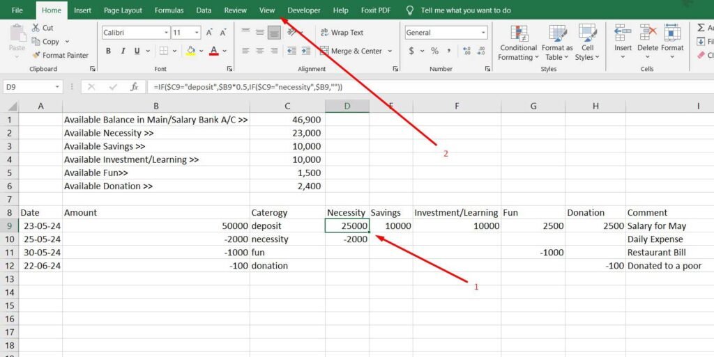
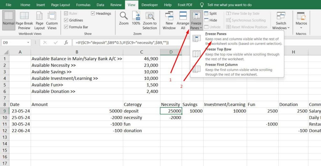 From now on, no matter how far you scroll down, the top section will remain visible.
 Dropdown
There are seven options in the category column to use: deposit, necessity, savings, investment, learning, fun, and donation. Instead of typing these each time, you can use the dropdown option to select from the seven choices.
To create the dropdown:
Select all the cells where you want to apply this feature. I have selected cells up to Row No. 100. I can repeat the process once these cells are filled.
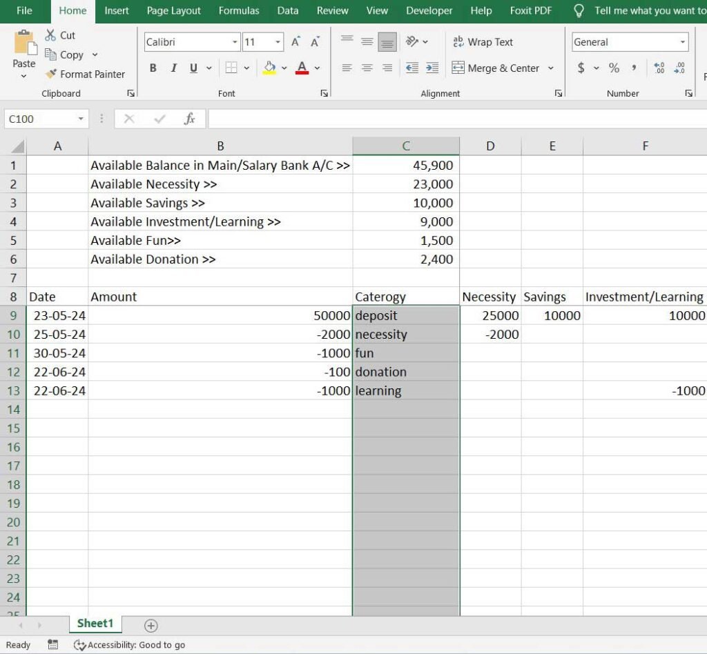
Click ‘Data’ from the menu and then select ‘Data Validation’.
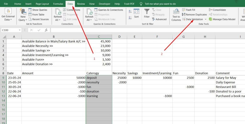
deposit,necessity,savings,investment,learning,fun,donation
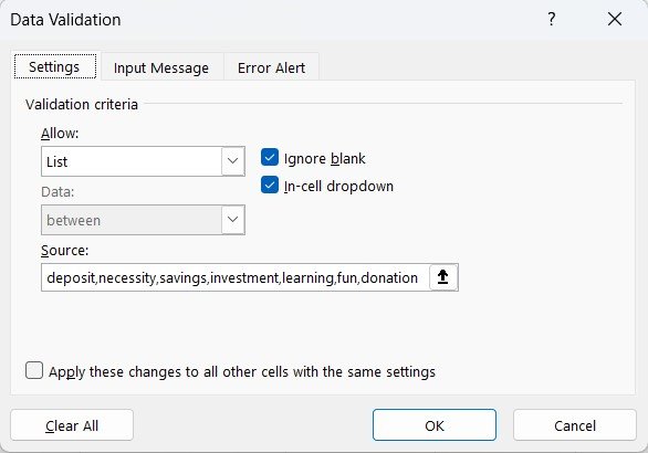
Click OK.
That’s it. Now, whenever you select a cell in the category column, a dropdown option will appear.
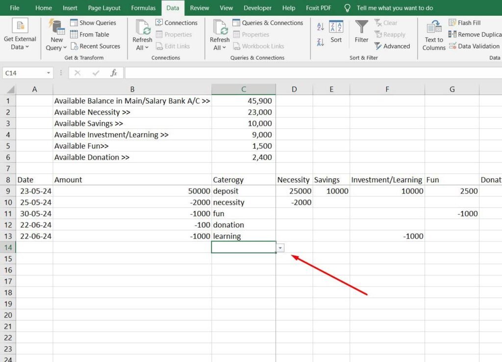
From here, you can choose your desired option.
Click here for the updated Excel file.

